See package website for full vignette
The Bioconductor build system does not have the MEME Suite installed, therefore these vignettes will not contain any R output. To view the full vignette, visit this article page on the memes website at this link
suppressPackageStartupMessages(library(GenomicRanges))
suppressPackageStartupMessages(library(magrittr))
suppressPackageStartupMessages(library(universalmotif))
library(memes)
Inputs
FIMO searches input sequences for occurrances of a motif. runFimo() has two required inputs: fasta-format sequences, with optional genomic coordinate headers, and a set of motifs to detect within the input sequences.
Sequence Inputs:
Sequence input to runFimo() can be as a path to a .fasta formatted file, or as a Biostrings::XStringSet object. Unlike other memes functions, runFimo() does not accept a Biostrings::BStringSetList as input. This is to simplify ranged join operations (see joins) on output data.
By default, runFimo() will parse genomic coordinates from sequence entries from the fasta headers. These are generated automatically if using get_sequences() to generate sequences for input from a GRanges object.
data("example_chip_summits", package = "memes")

dm.genome <- BSgenome.Dmelanogaster.UCSC.dm3::BSgenome.Dmelanogaster.UCSC.dm3

# Take 100bp windows around ChIP-seq summits
summit_flank <- example_chip_summits %>%
  plyranges::anchor_center() %>%
  plyranges::mutate(width = 100)

# Get sequences in peaks as Biostring::BStringSet
sequences <- summit_flank %>%
  get_sequence(dm.genome)

# get_sequence includes genomic coordinate as the fasta header name
names(sequences)[1:2]
#> [1] "chr3L:40482-40581" "chr3L:49795-49894"
Motif Inputs:
Motif input to runFimo() can be as a path to a .meme formatted file, a list of universalmotif objects, or a singular universalmotif object. runFimo() will not use any of the default search path behavior for a motif database as in runAme() or runTomTom().
e93_motif <- MotifDb::MotifDb %>%
  # Query the database for the E93 motif using it's gene name
  MotifDb::query("Eip93F") %>%
  # Convert from motifdb format to universalmotif format
  universalmotif::convert_motifs() %>%
  # The result is a list, to simplify the object, return it as a single universalmotif
  .[[1]]
#> See system.file("LICENSE", package="MotifDb") for use restrictions.

# Rename the motif from it's flybase gene number to a more user-friendly name
e93_motif["name"] <- "E93_FlyFactor"
Note about default settings
runFimo() is configured to use different default behavior relative to the commandline and MEME-Suite Server versions. By default, runFimo() runs using text mode, which greatly increases speed and allows returning all detected matches to the input motifs. By default runFimo() will add the sequence of the matched region to the output data; however, this operation can be very slow for large sets of regions and can drastically increase the size of the output data. To speed up the operation and decrease data size, set skip_matched_sequence = TRUE. Sequence information can be added back later using add_sequence().
fimo_results <- runFimo(sequences, e93_motif)Data integration with join operations
The plyranges package provides an extended framework for performing range-based operations in R. While several of its utilities are useful for range-based analyses, the join_ functions are particularly useful for integrating FIMO results with input peak information. A few common examples are briefly highlighted below:
plyranges::join_overlap_left() can be used to add peak-level metadata to motif position information:
fimo_results_with_peak_info <- fimo_results %>%
  plyranges::join_overlap_left(summit_flank)

fimo_results_with_peak_info[1:5]
#> GRanges object with 5 ranges and 9 metadata columns:
#>       seqnames        ranges strand |      motif_id           motif_alt_id
#>          <Rle>     <IRanges>  <Rle> |   <character>            <character>
#>   [1]    chr3L   66310-66321      - | E93_FlyFactor Eip93F_SANGER_10_FBg..
#>   [2]    chr3L 138527-138538      - | E93_FlyFactor Eip93F_SANGER_10_FBg..
#>   [3]    chr3L 384344-384355      - | E93_FlyFactor Eip93F_SANGER_10_FBg..
#>   [4]    chr3L 714116-714127      - | E93_FlyFactor Eip93F_SANGER_10_FBg..
#>   [5]    chr3L 714145-714156      - | E93_FlyFactor Eip93F_SANGER_10_FBg..
#>           score    pvalue    qvalue matched_sequence          id
#>       <numeric> <numeric> <numeric>      <character> <character>
#>   [1]     14.25  1.01e-05        NA     CCGGCCGAAAAT   peak_4627
#>   [2]     10.10  8.96e-05        NA     CTGTCCAAAAAT   peak_4647
#>   [3]     10.87  6.65e-05        NA     GCCGCCGAAAAA   peak_4670
#>   [4]     12.90  2.43e-05        NA     CGTGCCAAAAAT   peak_4752
#>   [5]     10.25  8.51e-05        NA     CTTCCCAAAAAA   peak_4752
#>       peak_binding_description e93_sensitive_behavior
#>                    <character>            <character>
#>   [1]                  ectopic                 Static
#>   [2]                   orphan                 Static
#>   [3]                   orphan             Decreasing
#>   [4]                  entopic                 Static
#>   [5]                  entopic                 Static
#>   -------
#>   seqinfo: 2 sequences from an unspecified genome; no seqlengths
plyranges::intersect_() can be used to simultaneously subset input peaks to the ranges overlapping motif hits while appending motif-level metadata to each overlap.
input_intersect_hits <- summit_flank %>%
  plyranges::join_overlap_intersect(fimo_results)

input_intersect_hits[1:5]
#> GRanges object with 5 ranges and 9 metadata columns:
#>       seqnames        ranges strand |          id peak_binding_description
#>          <Rle>     <IRanges>  <Rle> | <character>              <character>
#>   [1]    chr3L   66310-66321      * |   peak_4627                  ectopic
#>   [2]    chr3L 138527-138538      * |   peak_4647                   orphan
#>   [3]    chr3L 384344-384355      * |   peak_4670                   orphan
#>   [4]    chr3L 714116-714127      * |   peak_4752                  entopic
#>   [5]    chr3L 714145-714156      * |   peak_4752                  entopic
#>       e93_sensitive_behavior      motif_id           motif_alt_id     score
#>                  <character>   <character>            <character> <numeric>
#>   [1]                 Static E93_FlyFactor Eip93F_SANGER_10_FBg..     14.25
#>   [2]                 Static E93_FlyFactor Eip93F_SANGER_10_FBg..     10.10
#>   [3]             Decreasing E93_FlyFactor Eip93F_SANGER_10_FBg..     10.87
#>   [4]                 Static E93_FlyFactor Eip93F_SANGER_10_FBg..     12.90
#>   [5]                 Static E93_FlyFactor Eip93F_SANGER_10_FBg..     10.25
#>          pvalue    qvalue matched_sequence
#>       <numeric> <numeric>      <character>
#>   [1]  1.01e-05        NA     CCGGCCGAAAAT
#>   [2]  8.96e-05        NA     CTGTCCAAAAAT
#>   [3]  6.65e-05        NA     GCCGCCGAAAAA
#>   [4]  2.43e-05        NA     CGTGCCAAAAAT
#>   [5]  8.51e-05        NA     CTTCCCAAAAAA
#>   -------
#>   seqinfo: 2 sequences from an unspecified genome; no seqlengths
Identifying matched sequence
When setting skip_match_sequence = TRUE, FIMO does not automatically return the matched sequence within each hit. These sequences can be easily recovered in R using add_sequence() on the FIMO results GRanges object.
fimo_results_with_seq <- fimo_results %>%
  plyranges::join_overlap_left(summit_flank) %>%
  add_sequence(dm.genome)
Returning the sequence of the matched regions can be used to re-derive PWMs from different match categories as follows (here done for different binding categories):
motifs_by_binding <- fimo_results_with_seq %>%
  # Split on parameter of interest
  split(mcols(.)$peak_binding_description) %>%
  # Convert GRangesList to regular list() to use `purrr`
  as.list() %>%
  # imap passes the list entry as .x and the name of that object to .y
  purrr::imap(~{
    # Pass the sequence column to create_motif to generate a PCM
    create_motif(.x$sequence,
                 # Append the binding description to the motif name
                 name = paste0("E93_", .y))
    })
Motifs from each category can be visualized with universalmotif::view_motifs()
motifs_by_binding %>%
  view_motifs()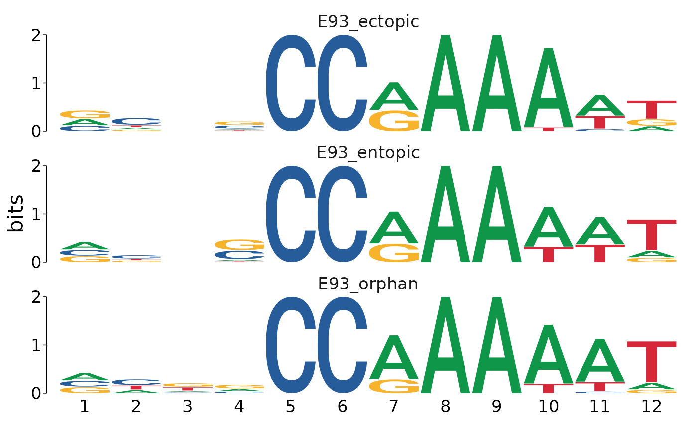
To allow better comparison to the reference motif, we can append it to the list as follows:
motifs_by_binding <- c(
  # Add the E93 FlyFactor motif to the list as a reference
  list("E93_FlyFactor" = e93_motif),
  motifs_by_binding
)
Visualizing the motifs as ICMs reveals subtle differences in E93 motif sequence between each category.
motifs_by_binding %>%
  view_motifs()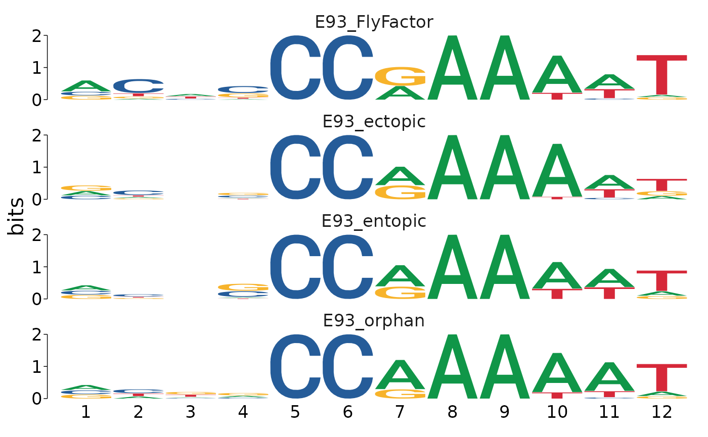
Visualizing the results as a position-probability matrix (PPM) does a better job of demonstrating that the primary differences between each category are coming from positions 1-4 in the matched sequences.
motifs_by_binding %>%
  view_motifs(use.type = "PPM")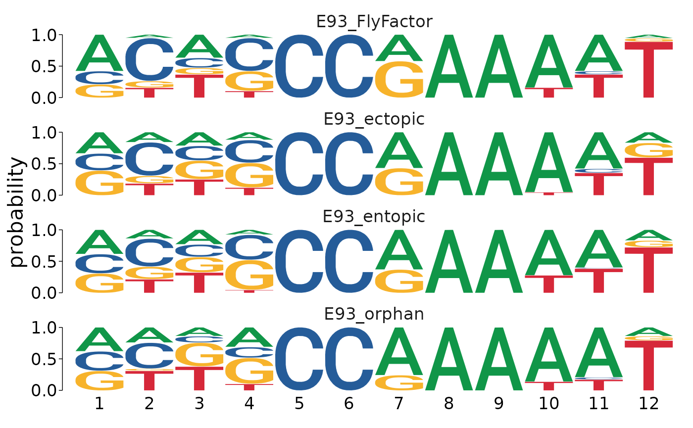
Finally, the sequence-level information can be used to visualize all sequences and their contribution to the final PWM using plot_sequence_heatmap.
plot_sequence_heatmap(fimo_results_with_seq$sequence)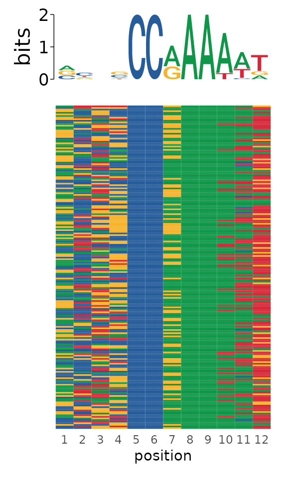
Importing Data from previous FIMO Runs
importFimo() can be used to import an fimo.tsv file from a previous run on the MEME server or on the commandline. Details for how to save data from the FIMO webserver are below.
Saving data from FIMO Web Server
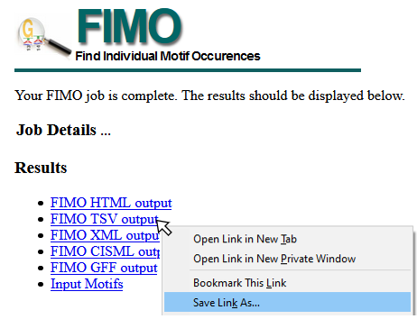
To download TSV data from the FIMO Server, right-click the FIMO TSV output link and “Save Target As” or “Save Link As” (see example image below), and save as <filename>.tsv. This file can be read using importFimo().
Citation
memes is a wrapper for a select few tools from the MEME Suite, which were developed by another group. In addition to citing memes, please cite the MEME Suite tools corresponding to the tools you use.
If you use runFimo() in your analysis, please cite:
Charles E. Grant, Timothy L. Bailey, and William Stafford Noble, “FIMO: Scanning for occurrences of a given motif”, Bioinformatics, 27(7):1017-1018, 2011. full text
Licensing Restrictions
The MEME Suite is free for non-profit use, but for-profit users should purchase a license. See the MEME Suite Copyright Page for details.
Session Info
sessionInfo()
#> R version 4.1.0 (2021-05-18)
#> Platform: x86_64-pc-linux-gnu (64-bit)
#> Running under: Ubuntu 20.04.3 LTS
#>
#> Matrix products: default
#> BLAS/LAPACK: /usr/lib/x86_64-linux-gnu/openblas-pthread/libopenblasp-r0.3.8.so
#>
#> locale:
#>  [1] LC_CTYPE=en_US.UTF-8       LC_NUMERIC=C
#>  [3] LC_TIME=en_US.UTF-8        LC_COLLATE=en_US.UTF-8
#>  [5] LC_MONETARY=en_US.UTF-8    LC_MESSAGES=C
#>  [7] LC_PAPER=en_US.UTF-8       LC_NAME=C
#>  [9] LC_ADDRESS=C               LC_TELEPHONE=C
#> [11] LC_MEASUREMENT=en_US.UTF-8 LC_IDENTIFICATION=C
#>
#> attached base packages:
#> [1] stats4    stats     graphics  grDevices utils     datasets  methods
#> [8] base
#>
#> other attached packages:
#> [1] memes_1.3.2           universalmotif_1.13.4 magrittr_2.0.1
#> [4] GenomicRanges_1.46.1  GenomeInfoDb_1.30.0   IRanges_2.28.0
#> [7] S4Vectors_0.32.3      BiocGenerics_0.40.0
#>
#> loaded via a namespace (and not attached):
#>  [1] bitops_1.0-7                          matrixStats_0.61.0
#>  [3] fs_1.5.1                              bit64_4.0.5
#>  [5] rprojroot_2.0.2                       tools_4.1.0
#>  [7] bslib_0.3.1                           utf8_1.2.2
#>  [9] R6_2.5.1                              splitstackshape_1.4.8
#> [11] colorspace_2.0-2                      withr_2.4.3
#> [13] processx_3.5.2                        tidyselect_1.1.1
#> [15] bit_4.0.4                             compiler_4.1.0
#> [17] textshaping_0.3.6                     Biobase_2.54.0
#> [19] desc_1.4.0                            DelayedArray_0.20.0
#> [21] labeling_0.4.2                        rtracklayer_1.54.0
#> [23] sass_0.4.0                            scales_1.1.1
#> [25] readr_2.1.1                           pkgdown_2.0.1.9000
#> [27] systemfonts_1.0.3                     stringr_1.4.0
#> [29] digest_0.6.29                         Rsamtools_2.10.0
#> [31] rmarkdown_2.11                        R.utils_2.11.0
#> [33] XVector_0.34.0                        pkgconfig_2.0.3
#> [35] htmltools_0.5.2                       MatrixGenerics_1.6.0
#> [37] highr_0.9                             fastmap_1.1.0
#> [39] BSgenome_1.62.0                       rlang_0.4.12
#> [41] farver_2.1.0                          BSgenome.Dmelanogaster.UCSC.dm3_1.4.0
#> [43] jquerylib_0.1.4                       BiocIO_1.4.0
#> [45] generics_0.1.1                        jsonlite_1.7.2
#> [47] vroom_1.5.7                           BiocParallel_1.28.2
#> [49] dplyr_1.0.7                           R.oo_1.24.0
#> [51] RCurl_1.98-1.5                        GenomeInfoDbData_1.2.7
#> [53] patchwork_1.1.1                       Matrix_1.3-4
#> [55] Rcpp_1.0.7                            waldo_0.3.1
#> [57] munsell_0.5.0                         fansi_0.5.0
#> [59] lifecycle_1.0.1                       R.methodsS3_1.8.1
#> [61] stringi_1.7.6                         yaml_2.2.1
#> [63] MASS_7.3-54                           SummarizedExperiment_1.24.0
#> [65] zlibbioc_1.40.0                       grid_4.1.0
#> [67] ggseqlogo_0.1                         parallel_4.1.0
#> [69] crayon_1.4.2                          lattice_0.20-44
#> [71] Biostrings_2.62.0                     hms_1.1.1
#> [73] ps_1.6.0                              knitr_1.36
#> [75] pillar_1.6.4                          rjson_0.2.20
#> [77] pkgload_1.2.4                         XML_3.99-0.8
#> [79] glue_1.5.1                            evaluate_0.14
#> [81] data.table_1.14.2                     vctrs_0.3.8
#> [83] tzdb_0.2.0                            testthat_3.1.0
#> [85] gtable_0.3.0                          purrr_0.3.4
#> [87] tidyr_1.1.4                           cachem_1.0.6
#> [89] ggplot2_3.3.5                         xfun_0.28
#> [91] restfulr_0.0.13                       ragg_1.2.0
#> [93] MotifDb_1.36.0                        tibble_3.1.6
#> [95] GenomicAlignments_1.30.0              plyranges_1.14.0
#> [97] memoise_2.0.1                         cmdfun_1.0.2
#> [99] ellipsis_0.3.2